“Success is stumbling from failure to failure with no loss of enthusiasm.”
— Winston Churchill
But that raises a natural question: how many times might I have to fail before I succeed?
That’s where the geometric distribution comes in. It’s the mathematical model that tells us the probability of achieving the first success after a series of independent failures.
The geometric distribution gives the probability that your first success occurs on the kth trial:
![]()
Where:
X = number of trials until the first success
p = probability of success in a single trial
(1−p)= probability of failure
Example: Rolling a 6 in Snakes and Ladders
Imagine you’re playing Snakes and Ladders, and you can only win if you roll a 6.
You want to know the probability that you’ll roll your first 6 on the fourth roll.
P(X= 4) = ( 1−1/6)^3 * 1/6
= (5/6)^3 * 1/6
= 0.096
So, there’s about a 9.6% chance that your first “6” will appear on the fourth try.
Expected Value (Mean)
The mean of the geometric distribution is:
E[X] = 1/p
This represents the average number of trials you’ll need to get your first success.
Example:
If p=0.2 then E[X ] = 1/0.2 = 5 , On average, you’ll succeed on the 5th trial.
For our die example, p = 1/6
E[X] = 1/1/6 = 6
Interpretation:
On average, you’ll need 6 rolls to get your first
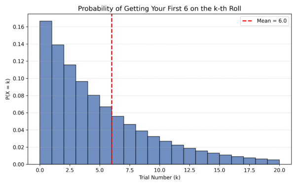
Sometimes it’ll happen sooner, sometimes later—but 6 is the expected number across many trials.
On average, you will need 6 rolls to get your first 6. Of course, that doesn’t mean you’ll magically roll a 6 every sixth time like clockwork. Some days, luck smiles early—you roll a 6 on the first try and feel like a wizard. Other times, the die acts like it’s personally offended and makes you wait 10 rolls.
But if you played this game a lot (say, hundreds or thousands of times), the average number of rolls before a 6 would settle nicely around 6. That’s the beauty of probability—it smooths out the chaos of luck over the long run.
Variance
The variance of a geometric distribution is:

This measures how spread out the number of trials is around the mean.
If p=0.2 then
Var(X) = 1 − 0.2/0.2^2 = 0.8 / 0.04 = 20
Why Variance Is Important
The geometric distribution models waiting time until the first success.
Its variance tells us how consistent or variable that waiting time might be.
Measures dispersion: While the mean tells the average waiting time, variance shows how much the actual trials fluctuate.
Predicts reliability: Low variance → predictable results. High variance → outcomes vary widely.
Guides decision-making: In quality control, marketing campaigns, or medical testing, high variance means more uncertainty in how long it takes to get success.
Shapes the curve: Higher variance → longer right tail (more extreme outcomes possible).
Connects to standard deviation: The square root of variance gives the standard deviation, which is often easier to interpret in practical terms (e.g., “on average, we’re off by X trials”).
As p increases (success becomes more likely), variance decreases — success happens sooner and more predictably. As p decreases (success is rare), variance increases — you might wait longer, and the timing of success becomes more uncertain.
The geometric distribution is more than just a probability formula—it’s a quiet reminder that persistence pays off. Each failed attempt isn’t wasted effort; it’s part of the journey that statistically moves you closer to success. The math might be about random trials, but the message is deeply human: keep rolling, keep trying—your first win could be just one more attempt away!