Have you ever felt like , statistics is just a jumble of confusing abbreviations? PDF, PMF, CDF — it’s enough to make you wonder if statisticians were too lazy to spell things out or they were just trying to make game of scrabble easier. Spoiler alert: PDF isn’t about Adobe, PMF has nothing to do with your pension, and CDF isn’t a sitcom from the ’90s. These acronyms are the unsung heroes of probability theory — the tools that help us make sense of randomness, uncertainty, and data-driven decisions.
In this post, we’ll unpack each one — with intuition, equations, and visuals — so you can finally see how they shape the story your data is trying to tell.
Let’s start with something simple: what you can count and what you can’t. That basic distinction is the foundation of what we’re about to explore. The Probability Mass Function (PMF) applies to discrete random variables — things you can count, like the outcome of rolling a fair die or the number of children in a family. Some examples are straightforward, but others can be surprisingly personal. Take a chocolate, for instance. To me, a piece of chocolate is always a discrete random variable. Why? Because I don’t share it with anyone — and I certainly don’t accept half a chocolate bar from anyone either. If it’s not a whole piece, it doesn’t count!
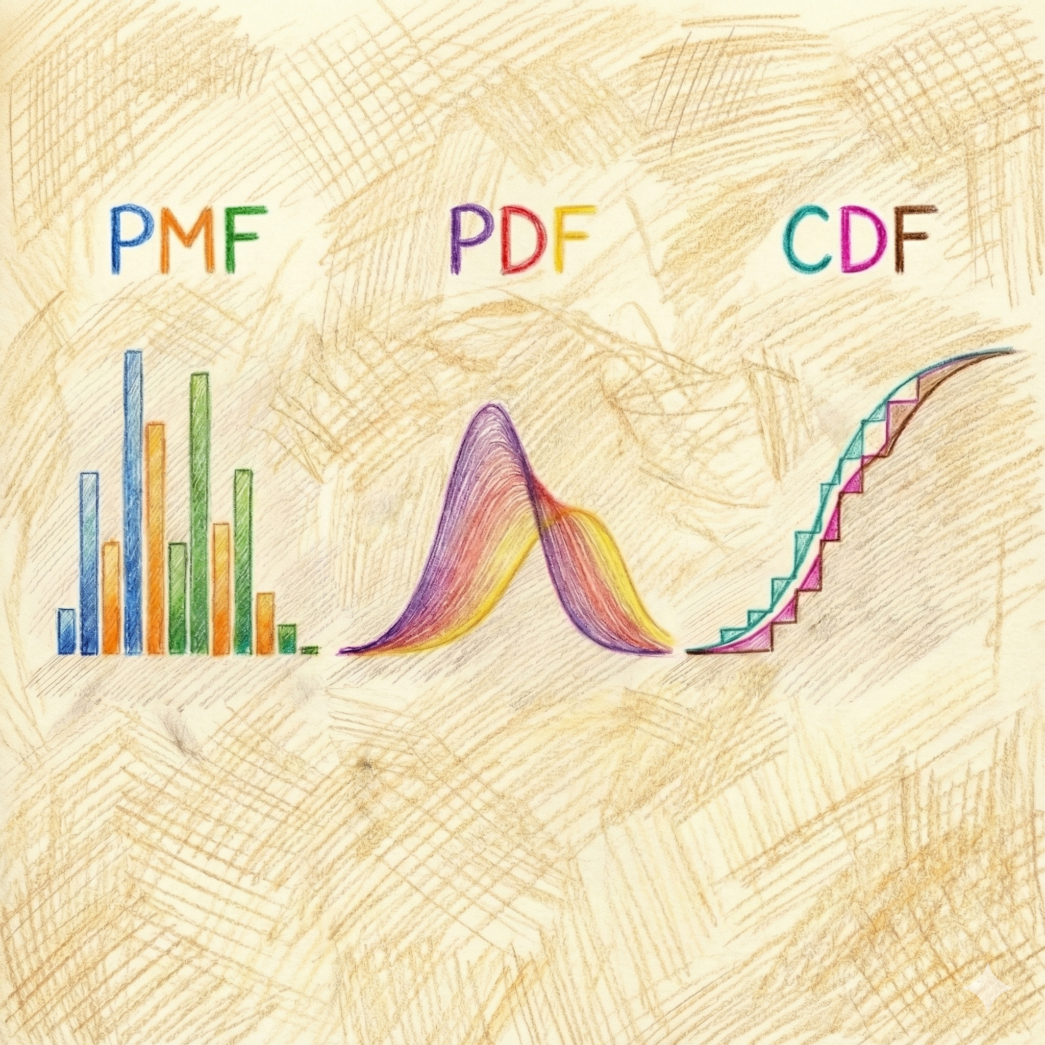
PMF: Probability Mass Function
The Probability Mass Function (PMF) applies to discrete random variables — outcomes that come in distinct, countable chunks. No half steps, no fractions in between.
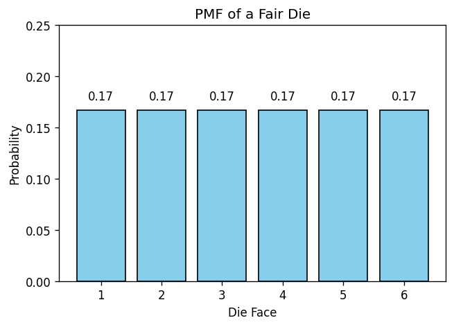
Think of rolling a die. You can’t roll a 2.5; your result must be one of the six whole numbers: 1, 2, 3, 4, 5, or 6. The PMF tells us the probability of each possible outcome.
For a fair die, each face is equally likely, so the PMF is simple:
In other words, every roll has a one-in-six chance — a neat, uniform distribution across all outcomes.
Discrete Distributions Under the PMF Framework: Binomial, Poisson, and Geometric
Distributions that fall under the PMF club are all about countable outcomes — the kind you can literally tick off on your fingers (or toes, if the numbers get big). Each one has its own personality, but they all follow the same rule: probabilities stick to neat, whole-number outcomes. No half events allowed!
- Binomial distribution : The Binomial distribution keeps score of your wins across repeated trials — like goals in football, or successful job applications out of a batch.
- Poisson distribution: counts how many “rare but random” things happen in a fixed time or space — like earthquakes in a region, volcano eruptions in a decade, or how many buses arrive at exactly 8:00 a.m. at your stop (at exact 8:00 a.m. is a rare event, it may be 8:00:30 or 8:01:00, unless you are in Germany). Or, if you’re lucky, a job offer lands in your inbox with a 70% salary hike!
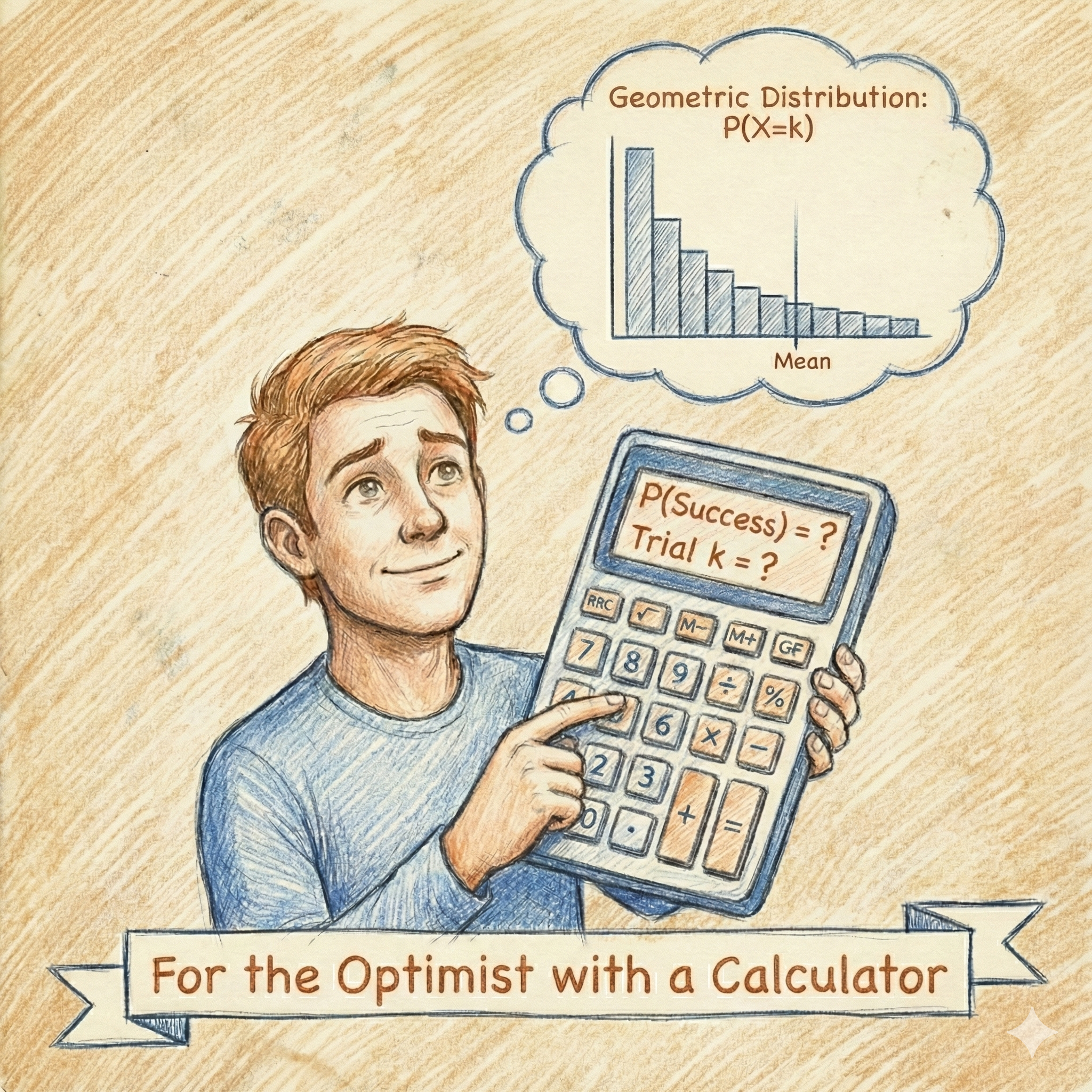
- Geometric distribution asks, “How many tries before you finally succeed?” — whether it’s rolling a six, finding a matching sock, or landing that dream job. In fact, how many more interviews before the Geometric distribution finally becomes the Poisson distribution?
Each distribution serves a different purpose but they all live by the same rule: probabilities stick to neat, whole-number outcomes – no half events allowed!

In the world of PMFs (Probability Mass Functions), we count things — discrete, separate, whole-number outcomes. Think dice rolls, shoe sizes, or the number of pets someone owns. But the PDF (Probability Density Function) world? That’s where we measure things that flow. Heights, weights, time, money, coffee temperature… these don’t come in tidy chunks; they slide smoothly along a scale.
A PDF doesn’t ask, “What’s the probability of being exactly 170.0 cm tall?” — because for continuous variables, the probability of any single, exact value is technically zero. Instead, it asks, “What’s the probability your height falls within a range, like between 169.5 cm and 170.5 cm?”
Think of it like raindrops sliding down a window: it spreads continuously across the number line. The curve might peak in some places and dip in others, but the total area under it always adds up to 1 — representing just a smooth, continuous trail that traces probability across the surface.
Caveat: While PDFs deal in continuous values, real-world data often gets rounded. For example, celebrity heights on Wikipedia are usually listed as whole numbers — not because people grow in 1 cm increments, but because that’s how we report and record them. The underlying reality is still continuous; the rounding is just a convenience.
Continuous Distributions Under the PDF Framework: Normal, Exponential, Lognormal, and Pareto
The PDF applies when outcomes are continuous—that is, they can take on infinitely many values within a range.
Example: Height. A person’s height could be 170.1 cm, 170.01 cm, 170.001 cm, and so on, with endless possibilities.
Here’s the tricky part: for continuous variables, the probability of hitting an exact value (say exactly 170.000 cm) is actually zero. Instead, we talk about the probability of landing in a range.
- A PDF is like a smooth curve that shows where values are more or less likely to occur.
- The area under the curve (not the height of the curve itself) tells us the probability.
- Example: “The probability that someone’s height is between 165 cm and 175 cm” = the area under the curve between those two numbers.
Think of PDF as a landscape. The taller the hill, the more likely values around that hill are to occur. But to get a probability, you always need to measure the area under the hill, not just the height.
Distributions that fall under the PDF (Probability Density Function) umbrella don’t bother with counting on your fingers — they operate in the smooth, continuous realm. These are the models for variables that flow rather than jump: time, height, income, temperature, and more.
Let’s meet a few key players:
- Normal Distribution: The superstar of the PDF world. This iconic bell curve shows up everywhere — from exam scores to human heights. It’s symmetric, centered, and beloved for its mathematical elegance.
- Exponential Distribution: Think of this one as your impatient friend, always asking, “How long until the next thing happens?” It models waiting times — like the time between bus arrivals or coffee orders.
- Lognormal Distribution: A bit sneakier. It hides in places like incomes and stock prices, where most values are modest, but a lucky few shoot way off the chart. It’s skewed, with a long tail of high values.
- Pareto Distribution: The classic “80/20 rule” in action. It explains why 20% of people might own 80% of the wealth — or 80% of the chocolate. It’s heavy-tailed and great for modeling inequality.
 we’ve seen how the PDF spreads probability across a continuous scale, But what if we want to know how much probability has accumulated up to a certain point? That’s where the Cumulative Distribution Function (CDF) steps in. If the PDF is about density, the CDF is about total.
CDF: Cumulative Distribution Function
Finally, the CDF is like a running total of probability.
Instead of asking, “What’s the probability of rolling a 3?” (PMF) or “What’s the probability someone’s height is between 165–175 cm?” (PDF), the CDF asks:
“What’s the probability the outcome is less than or equal to a certain value?”
Example with a die (PMF):
Probability(outcome ≤ 2) = P(1) + P(2) = 2/6
Probability(outcome ≤ 4) = P(1) + P(2) + P(3) + P(4) = 4/6
Example with height (PDF):
Probability(height ≤ 170 cm) = the area under the PDF curve from the far left up to 170.
The CDF always increases as you move right, starting at 0 (nothing less than the smallest possible value) and ending at 1 (certainty once you’ve included all possible values).
Summary:
PMF: for discrete outcomes; tells you the probability of each exact value.
PDF: for continuous outcomes; describes the shape of likelihood, where probabilities come from areas under the curve.
CDF: works for both; gives the probability of being less than or equal to a chosen value.