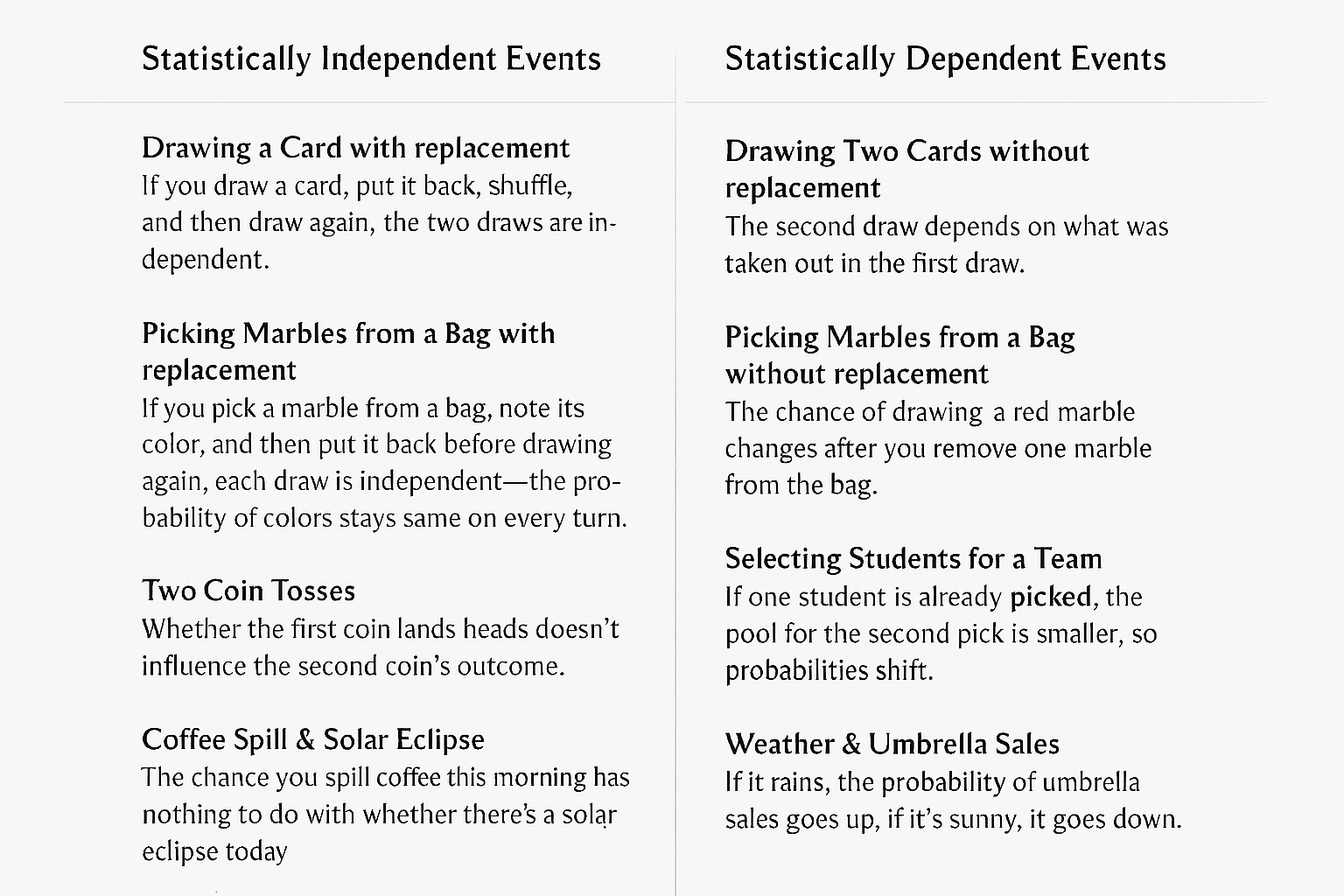
If you’ve ever felt lost in the world of probability — stumbling through Bayes’ theorem examples or getting tangled in those infamous ‘with replacement’ versus ‘without replacement’ questions — you’re not alone. The heart of the confusion often comes down to one pair of ideas: statistical independence and dependence. Grasping the difference between them isn’t just about solving textbook problems — it’s about building real intuition for how uncertainty works in the world around us. In this post, we’ll break them down clearly, with examples that finally make sense.
Probability has three main players you’ll see over and over again: marginal probability, joint probability, and conditional probability. Think of marginal probability as the solo act — the chance of a single event happening. Joint probability is the duet — two events happening together. And conditional probability is the twist — the chance of one event happening given that another has already occurred. In the next sections, we’ll see how each of these players behaves when the world is governed by independence versus when dependence quietly rewrites the rules.
Probabilities Under Statistical Independence:
Marginal Probability under Statistical Independence
Marginal probability is just the plain old probability of an event happening. When events don’t depend on each other, the marginal probability is simply the chance of that event on its own — no combos, no duets, just a solo performance.
For example, the probability of getting heads on a single coin toss is:
P(Head)= ½
And here’s the fun part: that never changes. Flip once, flip ten times, flip until your wrist hurts — the coin doesn’t care about your past results. Got five heads in a row? Cool story, but the next toss is still a clean 50/50. Each toss is independent, blissfully unaware of the others.
So we can say: “The outcome of each toss of a fair coin is statistically independent of every other toss.”
In short: toss once, toss twice, toss a hundred times — each flip is living in the moment. Yesterday’s tails have zero effect on today’s head.
Joint Probability of Independent Events (Multiplication Rule)
If marginal probability is just pressing play on Netflix, joint probability is pressing play and discovering a bag of chips in the cupboard.
The two events don’t depend on each other — Netflix doesn’t magically restock your snacks, and your chips don’t control your Wi-Fi. But together, they make the perfect combo.
And the math is just as simple as the vibe:
P(A∩B)=P(A)×P(B)
So, if the chance of your favorite show streaming smoothly is P(A), and the chance of finding chips is P(B), then the probability of Netflix + snacks night is just their product. Independent? Yes. Essential? Absolutely.
Coin tosses work the same way.
- Probability of heads on the first toss = ½
- Probability of heads on the second toss = 1/2
Since the tosses are independent, the joint probability of getting heads on both is:
P(Head on Toss 1 AND Head on Toss 2)=1/2 X 1/2
So there’s a 1 in 4 chance of scoring a double-head moment.
That’s joint probability of independent events: two worlds doing their own thing, but you still get to multiply them to see the odds of them colliding.
Conditional Probability of Independent Events
Conditional probability asks: “What’s the chance of A happening, given that B already happened?”
Now, picture this: you’re hungry and thinking about pizza delivery (Event A), and at the same time you’re hoping for sunny weather (Event B).
But here’s the kicker — pizza guys don’t check the sky before bringing your order, and the clouds don’t rearrange themselves based on your extra-cheese cravings. These two events are independent.
So the probability of getting your pizza given that it’s sunny is the same as the probability of getting your pizza on any random day:
P(Pizza | Sunny)=P(Pizza)
Formally, we write:
P(A∣B)=P(A∩B)/P(B)
Just like with coin tosses: the chance of getting heads on Toss 2 given Toss 1 was heads is still 1/2
Independence basically means: “Weather does weather. Pizza does pizza. Coins do coins.” No spoilers from one event to the other.
“Independent events mind their own business — what happens to one doesn’t change the odds of the other.
Probabilities Under Statistical Dependence:
Sometimes probabilities aren’t loners — they hang out in groups and influence each other. Statistical dependence happens when the chance of one event isn’t living on its own island, but actually shifts depending on whether another event shows up.
Scenario: The Ball Box Drama
Imagine a box stuffed with 20 balls: some are red, some are blue, some are green — and a few are rocking stripes while the rest are plain. Here’s the lineup:
|
Color |
Striped | Not Striped |
Total |
|
Red |
4 | 6 |
10 |
|
Blue |
3 | 2 |
5 |
|
Green |
2 | 3 |
5 |
|
Total |
9 | 11 |
20 |
Let’s name our events:
- S = ball is striped
- R = ball is red
Q1: What’s the probability a ball is striped, given that it’s red?
Think of it like this: once you peek at a ball and see red, the world shrinks to just the 10 red balls. Out of those, 4 wear stripes.
P(S∣R) = 4/10
= 0.4
So if you already know you’ve got a red ball, the odds of it being striped drop to 40%.
Q2: What’s the probability a ball is red, given that it’s striped?
Now flip the perspective. Pretend you only look at the 9 striped balls. Out of those, 4 are red.
P(R∣S) = 4/ 9
≈ 0.444
So about 44% of the striped crew are rocking red.
Joint Probabilities Under Statistical Dependence
Finally, what’s the chance that a ball is both red and striped in one go?
We chain things together:
P(R∩S) = P(R∣S)×P(S)
= 4/9×9/20
= 0.2
So only 20% of all balls in the box are part of the “red + striped” squad.
In short: unlike the coin flips (independence), here every choice reshuffles the story. The color you see changes how likely stripes are, and stripes change how likely color is. That’s the heartbeat of statistical dependence.
Marginal Probabilities under Statistical Dependence
Marginal probabilities are like the “big picture” view. Instead of zooming in on just one combo (like red and striped), you add up all the ways your event could happen.
Take red balls from our box example:
P(Red)=P(Red ∣ Striped)⋅P(Striped) + P(Red ∣ Not Striped)⋅P(Not Striped)
Crunching the numbers:
P(Red) = (4/9)(9/20)+(6/11)(11/20)
= 10/ 20
= 0.5
So half the box is red — and notice how we got there: by summing up the joint probabilities, not by treating events as totally independent.
Cheat Sheet: Independence vs. Dependence
| Type of Probability | Formula (Statistical Independence) |
Formula (Statistical Dependence) |
|
Marginal Probability |
P(A) |
Sum of all joint probabilities where A occurs =P(A∣B) P(B) + P(A∣B) P(B’) |
|
Joint Probability |
P(A∩B)=P(A) P(B) P(B∩A)=P(B) P(A) |
P(A∩B)=P(A∣B) P(B) P(B∩A)=P(B∣A) P(A) |
|
Conditional Probability |
P(A∣B)=P(A) P(B∣A)=P(B) |
P(A∣B)=P(A∩B)P(B) |
Try Independent events, Dependent Events, Without Replacement and With Replacement, Please Reset before changing the event type for the best experience.
Independence & Dependence Simulator
Two worlds, one big idea — does knowing one event change what you expect from another?
In independent events, conditional probability converges to marginal probability.
The coin has no memory. It doesn't know it landed heads last time — each flip starts completely fresh. No matter how many heads you've seen in a row, the next flip is still 50/50. This is called the Gambler's Fallacy when people believe otherwise.
When events are independent, knowing B happened tells you nothing new about A. The conditional probability equals the marginal probability — not eventually, but always. Notice the P(H) and P(H|prev H) cards above always show the same number.
P(H) = 0.5. P(H | prev H) = P(H) = 0.5 — always, instantly, not eventually. P(H∩H) = P(H) × P(H) = 0.5 × 0.5 = 0.25. The conditional never changes because the coin has no memory of past flips.
P(H | prev H) = P(H) • P(H∩H) = P(H) × P(H) • No memory, no influence, no change.