When we learn Linear Regression, how nice it would be, if we have to deal with just y = mx+c; easy to draw and easy to understand. But in the real world, we rarely predict things based on just one feature—we usually have dozens! Foolhardy me still wanted a way to visualize this in action, so I decided to use a concept I call the ‘composite intercept.’
Think of it like freezing the entire world to focus on one thing at a time. Here is the plan: I will vary one variable while keeping the others constant. Then, I’ll add the value of those constants to the intercept. This will let me focus on the variable and the weight I am changing. So, what I am going to do is take a 2-D cross-section of an n-dimensional space and visualize it. (Warning: In reality all n dimensions change individually, I am using composite intercept for visual simplicity, It is like in biology lab, we don’t put whole onion under the microscope to understand the cell structure rather we take cross-section of it and put that under the microscope, or In Engineering Drawing , most of the times, we have drawn cross sections of front view or top view)
I am going to analyze my electricity bill to see how my AC and dryer usage determine the cost.
Let’s say the following is the formula for predicting the total electricity bill(y):
y = x1.w1 + x2.w2 + w0
where:
- w0 (Bias/Intercept): $10 Fixed Monthly Fee.
- w1 (Weight 1): $2 per hour for AC.
- x1 (Feature 1): Hours the AC is running.
- w2 (Weight 2): $5 per load for the Dryer.
- x2 (Feature 2): Number of Dryer loads.
Let’s see how this works compare to y = mx+c , please look at the following table
|
Math Role (y=mx+c) |
View A: AC is the Star (Plotting AC Hours on X-Axis) | View B: Dryer is the Star (Plotting Dryer Loads on X-Axis) | |
| Input / Features (x) |
x1 (AC Hours) |
x2 (Dryer Loads) |
|
| Slope / Weights (m)
(The Rate) |
w1 (Cost of running AC ) |
w2 (Cost of loading a dryer load ) |
|
| Intercept (c)
(The Base Rate) |
w0 + w2x2
Fixed Fee + Dryer Cost |
w0 + w1x1 Fixed Fee + AC Cost |
Whether a term acts as a “Slope” or part of the “Intercept” depends entirely on which variable we are currently changing (the active input) and which ones we are holding constant (the background inputs).
Here is how the roles flip if we change our perspective.
- The Standard View (AC is Active)
We put AC Hours (x1) on the X-axis.
- Active Variable: x1 (AC)
- Slope: w1 (cost of running an AC) → Because this determines how the line rotates, as the AC usage increases.
- Intercept: w0+w2x2 → The Fixed Fee + The “Frozen” Dryer Cost.
- The “Flipped” View (Dryer is Active)
Imagine we decide to make a graph where the X-axis is Dryer Loads (x2), and we keep the AC running at a constant 5 hours in the background.
The equation rearranges like this:
y = Composite Intercept (w0 + w1⋅x1) + Slope (w2⋅x2)
Now, look at the roles:
- Active Variable: x2 (Dryer)
- Slope: w2 (Price of Dryer) → Now this controls the steepness.
- Composite Intercept: w0+w1x1 → The Fixed Fee (10) + The “Frozen” AC Cost (2×5 = 10).
I hope without me telling you , you must have realized something…Don’t you think ?This is very similar to partial derivatives in gradient descent! Not sure ? please read below.
In Gradient Descent, we need to know: “Which weight should I change, and how much, to lower the error?”
Since we have multiple weights (w0, w1, w2), you can’t just take one general “derivative” for all of them. we need to know the specific impact of each weight individually, assuming the others are constant.
Here is how our electricity bill example maps to partial derivatives:
The “Partial” Perspective:
When we calculate a Partial Derivative, we are mathematically doing exactly what we did in View A of your table:
- We freeze w0 and w2: We pretend they are constants (part of the intercept).
- We look only at w1: We ask, “If I change w1 slightly, does the Total bill (total error) go up or down?”
Gradient Descent collects these partial answers into a list called the Gradient: Just a vector! Which talks to the algorithm something like,”The slope is steep for the AC rate (w1), so change that a lot. But the slope is flat for the Dryer rate (w2), so don’t change that too much to lower the total bill aka total error.”
Without partial derivatives, the algorithm wouldn’t know which weight was causing the error, just like looking at a high bill and not knowing if it was the AC or the Dryer that caused it.
Back to the Linear Regression!
We are going to visualize only View A. I will keep AC hours on the x-axis and Dryers load as “held-constant”, just to show that constants don’t disappear in a multidimensional world, but they act as hidden choices.
View A: AC is the Star (Plotting AC Hours on X-Axis)
Scenario 1: Cutting AC Hours
The Situation: We decide to save money by turning off the Air Conditioner. We reduce usage from 10 hours down to 0 hours. The price of electricity hasn’t changed, and we still do our normal laundry (3 loads).
The Variables:
x1 (AC Hours): Changes from 10 → 0
x2 (Dryer Loads): Fixed at 3
Weights (w0,w1,w2): Fixed (Prices don’t change)
Manual Calculation:
- Start (10 Hours):
w0 (Bias/Intercept): $10 Fixed Monthly Fee.
w1 (Weight 1): $2 per hour for AC.
x1 (Feature 1): 5 hours of running an AC
w2 (Weight 2): $5 per load for the Dryer.
x2 (Feature 2): Number of Dryer loads.
w0 + x1w1 + x2w2 = y
10 + (2×10) + (5×3) = 10 + 20 + 15 = $45
- End (0 Hours):
x1 (Feature 1): 0 hours of running an AC
10+ (2×0) + (5×3) = 10 + 0 + 15 = $25
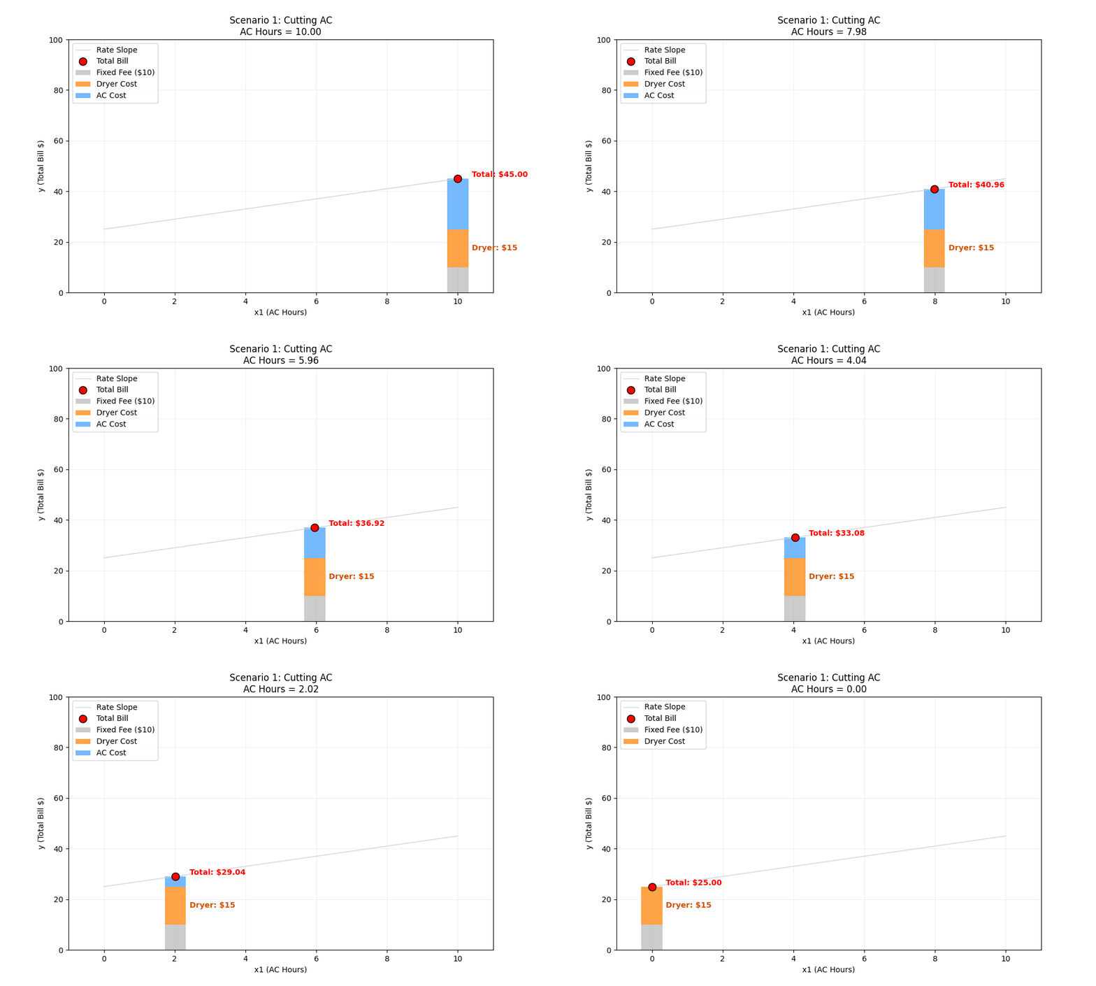
ML Intuition (Movement Along the Line): Because our graph’s X-axis is “AC Hours” (x1), changing x1 just means moving the red dot along the existing line. The slope (rate) and the intercept (base cost) stay exactly the same.
Scenario 2: Stopping the Dryer
The Situation: We keep the AC running for 5 hours, but We stop using the Dryer completely (reducing loads from 5 to 0).
The Variables:
x1 (AC Hours): Fixed at 5
x2 (Dryer Loads): Changes from 5 → 0
Weights (w0,w1,w2): Fixed
Manual Calculation:
- Start (5 Loads):
w0 (Bias/Intercept): $10 Fixed Monthly Fee.
w1 (Weight 1): $2 per hour for AC.
x1 (Feature 1): 5 hours of running an AC
w2 (Weight 2): $5 per load for the Dryer.
x2 (Feature 2): 5 Dryer loads
10 + (2×5) + (5×5) = 10 + 10 + 25 = $45
- End (0 Loads):
x2 (Feature 2): 0 Dryer loads
10 + (2×5) + (5×0) = 10 + 10 + 0 = $20
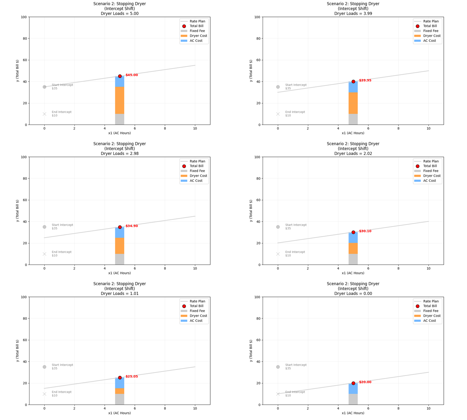
ML Intuition (The Intercept Shift): In our graph, the X-axis is AC Hours (x1). The Dryer (x2) is a “held-constant” variable. When you change a variable that is being held constant, it changes the Composite Intercept.
- Start Intercept: Fixed Fee (10) + Dryer Cost (25) = 35
- End Intercept: Fixed Fee (10) + Dryer Cost (0) = 10
Visually, the entire line shifts down. The slope (steepness) doesn’t change because the AC rate didn’t change.
Scenario 3: The AC Price Hike
The Situation: The power company gets greedy. They raise the price of running the AC from $2/hour to $8/hour. our usage stays the same.
The Variables:
- x1,x2 (Usage): Fixed (5 hours, 3 loads)
- w1 (AC Rate): Changes from 2 → 8
- w0,w2: Fixed
Manual Calculation:
- Start ($2 Rate):
w0 (Bias/Intercept): $10 Fixed Monthly Fee.
w1 (Weight 1): $2 per hour for AC.
x1 (Feature 1): 5 hours of running an AC
w2 (Weight 2): $5 per load for the Dryer.
x2 (Feature 2): Number of Dryer loads.
10 + (2×5) + (5×3) = 10 + 10 + 15 = $35
- End ($8 Rate):
w1 (Weight 1): $8 per hour for AC.
10 + (8×5) + (5×3) = 10 + 40 + 15 = $65
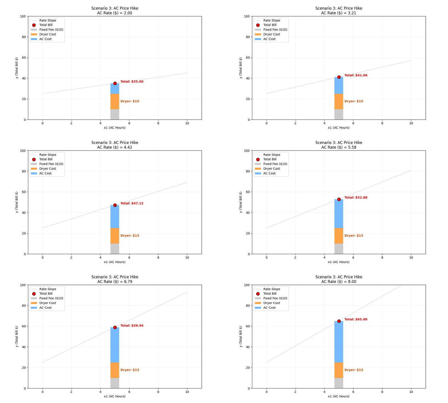
ML Intuition (Slope Change): w1 represents the relationship between the X-axis (x1) and the Y-axis (Bill). When w1 increases, the output becomes much more sensitive to the input. Visually, the line rotates and becomes steeper. A small change in AC hours now leads to a massive change in the bill.
Scenario 4: The Dryer Price Hike
The Situation: The power company raises the cost of running the Dryer from $5/load to $15/load. Our usage is 3 loads of laundry.
The Variables:
- x1, x2 (Usage): Fixed (5 hours, 3 loads)
- w2 (Dryer Rate): Changes from 5 → 15
- w0,w1: Fixed
Manual Calculation:
- Start ($5 Rate):
w0 (Bias/Intercept): $10 Fixed Monthly Fee.
w1 (Weight 1): $2 per hour for AC.
x1 (Feature 1): Hours the AC is running.
w2 (Weight 2): $5 per load for the Dryer.
x2 (Feature 2): Number of Dryer loads.
10 + (2×5) + (5×3) = 10 + 10 + 15 = $35
- End ($15 Rate):
w2 (Weight 2): $15 per load for the Dryer.
10 + (2×5) + (15×3) = 10 + 10 + 45 = $65

ML Intuition (Weight-Driven Intercept Shift): This looks very similar to Scenario 2, but the cause is different. Usually, we think of weights (w) as controlling rotation (slope). But here, increasing a weight (w2) causes a vertical shift (intercept). Why?
- In Scenario 2, the Input/feature (x2) changes
- In Scenario 4, the Weight (w2) changes
Context Matters: Because the Dryer (x2) is not on our X-axis, the model sees the entire cost of the dryer (w2*x2) as a fixed “surcharge” or starting cost. As It gets added into the Composite Intercept.
The Multiplier Effect : This is different from just raising the fixed monthly fee (w0). The magnitude of the jump depends on your usage (x2).
- If you did 0 loads of laundry, this price hike wouldn’t affect you at all (the line wouldn’t move).
- Because you do 3 loads, the price hike is multiplied by 3. A $10 rate increase becomes a $30 jump in the intercept.
Visual Result: Since the AC rate (w1) didn’t change, the “steepness” of the line remains identical. The relationship between AC usage and the bill is unchanged; the line simply “floats” higher parallel to the original.
